Getting and Installing SNNS

Conventional algorithmic solution methods require the application of unambiguous definitions and procedures. This requirement makes them impractical or unsuitable for applications such as image or sound recognition where logical rules do not exist or are difficult to determine. These methods are also unsuitable when the input data may be incomplete or distorted. Neural networks provide an alternative to algorithmic methods. Their design and operation is loosely modeled after the networks of neurons connected by synapses found in the human brain and other biological systems. One can also find neural networks referred to as artificial neural networks or artificial neural systems. Another designation that is used is “connectionism”, since it deals with information processing carried out by interconnected networks of primitive computational cells. The purpose of this article is to introduce the reader to neural networks in general and to the use of the Stuttgart Neural Network Simulator (SNNS).

In order to understand the significance of the ability of a neural network to handle data which is less than perfect, we will preview at this time a simple character-recognition application and demonstrate it later. We will develop a neural network that can classify a 7×5 rectangular matrix representation of alphabetic characters.

 

 

 

 

 

 

 

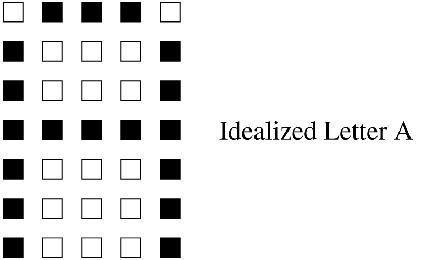
Figure 1. Ideal Letter “A”

In addition to being able to classify the representation in Figure 1 as the letter “A”, we would like to be able to do the same with Figure 2 even though it has an extra pixel filled in. As a typical programmer can see, conventional algorithmic solution methods would not be easy to apply to this situation.

 

 

 

 

 

 

 

 

 

 

 

 

 

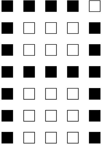
Figure 2. Blurred “A”

A neural network consists of an interconnected network of simple processing elements (PEs). Each PE is one of three types:

Connections exist between selected pairs of the PEs. These connections carry the output in the form of a real number from one element to all of the elements to which it is connected. Each connection is also assigned a numeric weight.

PEs operate in discrete time steps t. The operation of a PE is best thought of as a two-stage function. The first stage calculates what is called the net input, which is the weighted sum of its input elements and the weights assigned to the corresponding input connections. For the jth PE, the value at time t is calculated as follows:

 

 

where j identifies the PE in question, xi(t) is the input at time t from the PE identified by i, and wi,j are the weights assigned to the connections from i to j.

The second stage is the application of some output function, called the activation, to the weighted sum. This function can be one of any number of functions, and the choice of which one to use is dependent on the application. A commonly used one is known as the logistic function:

 

 

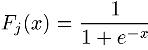
which always takes on values between 0 and 1. Generally, the activation Aj for the jth PE at time t+1 is dependent on the value for the weighted sum netj for time t:

 

 

In some applications, the activation for step t+1 may also be dependent on the activation from the previous step t. In this case, the activation would be specified as follows:

 

 

In order to help the reader make sense out of the above discussion, the illustration in Figure 3 shows an example network.

 

 

 

 

 

 

 

 

 

 

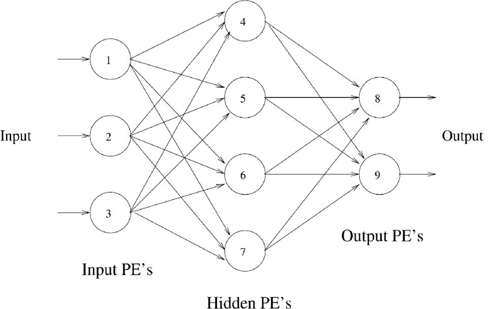
Figure 3. Sample Neural Network

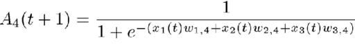
This network has input PEs (numbered 1, 2 and 3), output PEs (numbered 8 and 9) and hidden PEs (numbered 4, 5, 6 and 7). Looking at PE number 4, you can see it has input from PEs 1, 2 and 3. The activation for PE number 4 then becomes:

 

 

If the activation function is the logistic function as described above, the activation for PE number 4 then becomes

 

 

 

A typical application of this type of network would involve recognizing an input pattern as being an element of a finite set. For example, in a character-classification application, we would want to recognize each input pattern as one of the characters A through Z. In this case, our network would have one output PE for each of the letters A through Z. Patterns to be classified would be input through the input PEs and, ideally, only one of the output units would be activated with a 1. The other output PEs would activate with 0. In the case of distorted input data, we should pick the output with the largest activation as the network’s best guess.

The computing system just described obviously differs dramatically from a conventional one in that it lacks an array of memory cells containing instructions and data. Instead, its calculating abilities are contained in the relative magnitudes of the weights between the connections. The method by which these weights are derived is the subject of the next section.

In addition to being able to handle incomplete or distorted data, a neural network is inherently parallel. As such, a neural network can easily be made to take advantage of parallel hardware platforms such as Linux Beowulf clusters or other types of parallel processing hardware. Another important characteristic is fault tolerance. Because of its distributed structure, some of the processing elements in a neural network can fail without making the entire application fail.

In contrast to conventional computer systems which are programmed to perform a specific function, a neural network is trained. Training involves presenting the network with a series of inputs and the outputs expected in each case. The errors between the expected and actual outputs are used to adjust the weights so that the error is reduced. This process is typically repeated until the error is zero or very small.

Training methods vary greatly from one application to the next, and there is no single universal solution. As an example, we turn to a general discussion of what is known as gradient descent or steepest descent. Here, the error for each training pattern is quantified as:

 

 

 

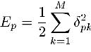
where Ep is the error for pattern p and

 

pk is the difference between the expected and actual outputs for pattern p and output PE k. The error Ep can also be thought of as a scalar valued function of the set of connection weights in the network:

 

 

With this in mind, minimizing Ep involves moving the weights in the direction of the negative gradient –

 

Ep. The weight change for a selected weight wi can be calculated as:

 

 

where nu is some constant between 0 and 1. The function F is typically chaotic and highly nonlinear. That being the case, the actual gradient component may be a very large value that may cause us to overshoot the solution. The constant nu can be used to suppress this.

I have included the above discussion mostly for the benefit of readers with some basic knowledge of multi-variable calculus. For others, it is really only important to know that, through an iterative process, a neural network is adapted to fit its problem domain. For this reason, neural networks are considered to be part of a larger class of computing systems known as adaptive systems.

Although the actual implementation and operation of a neural network can be accomplished on a variety of platforms ranging from dedicated special-purpose analog circuits to massively parallel computers, the most practical is a conventional workstation. Simulation programs could be written from scratch, but the designer can save much time by using one of several available neural network prototyping tools. One such tool is the Stuttgart Neural Network Simulator (SNNS).

The easiest way to get started with SNNS is to experiment with one of the example networks that comes with the distribution. One of these is a solution to the character recognition problem discussed at the beginning of this article.

Upon invoking SNNS, the manager (Figure 4) and banner (Figure 5) windows appear.

 

 

 

 

 

 

 

 

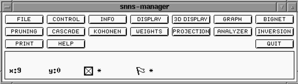
Figure 4. SNNS Manager

 

 

 

 

 

 

 

 

 

 

 

 

 

 

Figure 5. SNNS Banner

Selecting the file option from the manager window presents the user with a file selection box (Figure 6).

 

 

 

 

 

 

 

 

 

 

 

 

 

 

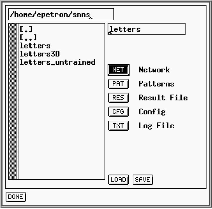
Figure 6. SNNS File Selection

The file selector uses extensions of .net, .pat, etc. to filter the file names in the selected directory. We will load the letters_untrained.net file, since we want to see the training process in action. We will also load the letters.cfg configuration file and the letters.pat file which contains training patterns.

After the files are loaded, selecting the display option in the manager window will present the user with a graphical display of the untrained network (Figure 7).

 

 

 

 

 

 

 

 

 

 

 

 

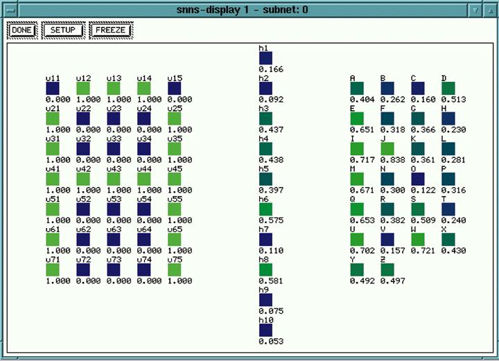
Figure 7. SNNS Untrained Network Display

This window shows the input units on the left, a layer of hidden units in the center and the output units on the right. The output units are labeled with the letters A through Z to indicate the classification made by the network. Note that in the Figure 7 display, no connections are showing yet because the network is untrained at this point.

 

 

 

 

 

 

 

 

 

 

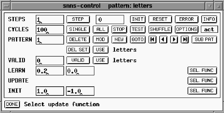
Figure 8. SNNS Control Window

Selecting the control option from the manager window presents the user with the control window (Figure 8). Training and testing are directed from the control window. Training basically involves the iterative process of inputting a training vector, measuring the error between the expected output and the actual output, and adjusting the weights to reduce the error. This is done with each training pattern, and the entire process is repeated until the error is reduced to an acceptable level. The button marked ALL repeats the weight adjustment process for the entire training data set for the number of times entered in the CYCLES window. Progress of the training can be monitored using the graph window (Figure 9).

 

 

 

 

 

 

 

 

 

 

 

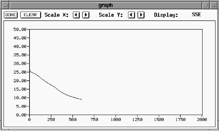
Figure 9. SNNS Graph Window

In the graph window, the horizontal axis shows the number of training cycles and the vertical axis displays the error.

 

 

 

 

 

 

 

 

 

 

 

 

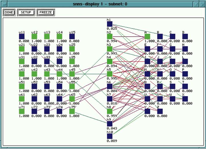
Figure 10. Partially Trained Network

Figure 10 shows a partially trained network. In contrast to the untrained network in Figure 7, this picture shows some connections forming. This picture was taken at the same time as Figure 9. After enough training repetitions, we get a network similar to that shown in Figure 11. Notice that the trained network, when the letter A is input on the left, the corresponding output unit on the right is activated with a 1.

 

 

 

 

 

 

 

 

 

 

 

 

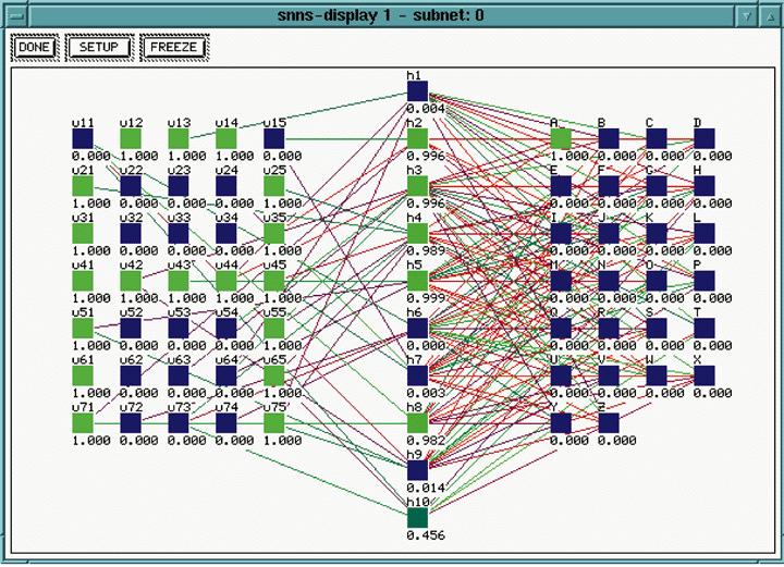
Figure 11. Trained Network

As a quick check to see if the network can generalize, a modified version of the training data set is tested with one of the dots in the A matrix set to zero instead of one, while an erroneous dot is set to one instead of zero. Figure 12 demonstrates that the distorted version of the letter A is still recognized.

 

 

 

 

 

 

 

 

 

 

 

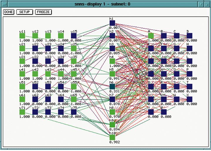
Figure 12. Test of Distorted A

As pointed out in the section on training, many different methods can be used to adjust the connection weights as part of the training process. The proper one to use depends on the application and is often determined experimentally. SNNS can apply one of many possible training algorithms automatically. The training algorithm can be selected from the drop-down menu connected to the control window.

SNNS reads network definition and configuration data from ASCII text files, which can be created and edited with any text editor. They can also be created by invoking the bignet option from the manager window. bignet enables the creation of a network by filling in general characteristics on a form. Refinements can be made by manually editing the data files with a text editor or by using other options within SNNS. Training and test data files are also plain ASCII text files.

Other notable features of SNNS include:

Complete instructions for getting and installing SNNS can be found at http://www.informatik.uni-stuttgart.de/ipvr/bv/projekte/snns/obtain.html. Prepackaged binaries are also available as part of the Debian distribution. Check http://www.debian.org/ for the Debian FTP site nearest you.

Neural networks enable the solution of problems for which there is no known algorithm or defining set of logical rules. They are based loosely on neurobiological processes and are thus capable of decisions which are intuitively obvious to humans but extremely difficult to solve using conventional computer processes. They are also less brittle and prone to failure than conventional systems due to their distributed nature. Their inherent parallelism provides opportunities for highly optimized performance using parallel hardware. The Stuttgart Neural Network Simulator (SNNS) is a powerful tool for prototyping computer systems based on neural network models.