Geomview

At first glance, Geomview appears to be a neat piece of 3-D software—a toy. In reality, an hour’s study of the program and the documentation will convince you that it is an extremely powerful visualization tool with virtually unlimited applications. With the mouse, you can easily rotate, scale, translate, and change the lighting of the objects. You can even “fly” through the scene using a built-in “flight simulator”.

These tools alone are enough to make Geomview worth loading onto your machine, but there is more. Incorporated into Geomview is a Graphical Command Language (GCL) which you can use to manipulate the 3-D objects in more ways than with the mouse alone. Additionally, you can pipe GCL commands into Geomview from other programs, allowing use of the package as a powerful interactive display for your own code.

Geomview was created at the University of Minnesota Geometry Center and was designed to serve as both a general purpose viewer and a visualization tool for mathematics research. Thus, the package also comes with the capability to display representations of 3-D objects as well as the ability to display objects in spherical and hyperbolic spaces. The package also includes code which allows you to use Geomview as the default 3-D viewer for Mathematica.

This article demonstrates how to create and animate objects in Geomview and tells you how to obtain a copy for yourself.

Geomview comes packed with loads of sample images in the Geomview/data directory. Getting started is as easy as typing geomview followed by the path and name of one of the image files. For example, Figure 1 shows the file

/usr/local/Geomview/data/geom/office.oogl

Figure 1

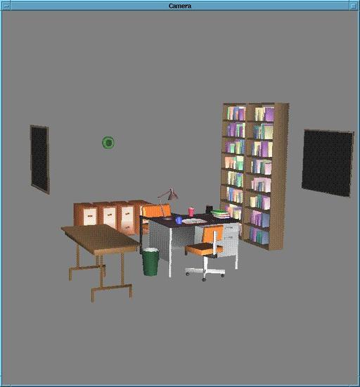
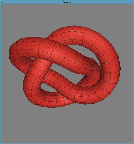
as well as the two other widgets that will appear on the screen when you first start Geomview. If you are running Geomview on a slower machine, you may notice that manipulating the somewhat complex scene of Figure 1 may be a little grueling. You may therefore want to start out with something a little simpler, like:

Geomview/data/things/dragon.off

or the trefoil knot

Geomview/data/things/trefoil_knot.mesh

which are shown in Figure 2.

Performing rotations, translations, and engaging the flight simulator are all pretty straight forward. For example, to rotate a scene displayed by the camera widget, just press the rotate button on the tools widget, and drag the mouse in the camera widget while holding down the left mouse button. The scene will rotate about an axis parallel to the camera window. If you let go of the left mouse button, the graphic will continue to spin with a speed proportional to the speed of the mouse when you released the button. (This option can be turned off in the motion menu by toggling to the inertia option if you desire a static view of the scene.) Translating and zooming are just as easy.

Rotating the scene may be a little awkward when you first start using Geomview; however, with a little practice, you will quickly get the hang of manipulating objects. It helps if you imagine that the objects displayed by the camera are contained in a giant imaginary sphere. The mouse is then a “gripper” which will latch onto the sphere when the left mouse button is clicked. Moving the mouse with the gripper engaged will cause the sphere to rotate about an axis parallel to the camera plane. To get another view of the scene, you can rotate about an axis perpendicular to the camera plane by using the middle mouse button to activate the middle gripper instead of the left one. The same applies for translations. To translate along an axis perpendicular to the screen, you use the center mouse button.

You can activate Geomview’s flight simulator by pressing the fly button in the tools menu, then dragging the mouse from the bottom of the camera widget to the top while holding down the middle mouse button. Again, the speed of your flight will depend on how fast you move the mouse. You can steer through the scene by dragging the mouse on the camera widget and clicking on the left or middle mouse buttons. If you want to stop the motion and take a serious look at something, you can press the halt button, located on the tools widget.

Browsing through the inspect menu on the Geomview widget, you will see a sample of the many attributes of the scene that can be selected and changed. Geomview does not limit you to just changing the color of the surfaces or the edges of the objects. It also allows you to control the color, the placement, and the intensity of the lights which illuminate the scene. There are a myriad other useful options which are fairly well described in the manual contained in the Geomview/doc directory.

The machinery of Geomview is contained within the Object Oriented Graphics Library (OOGL) which was also developed by the Geometry Center at the University of Minnesota. All of the scenes that are displayed by Geomview are described in terms of OOGL objects. For example, a sphere in Geomview can be described in terms of the OOGL object called SPHERE. The type of object, as well as the physical description, can be passed to Geomview in an OOGL object file which, in the case of a simple sphere, would contain the following text:

SPHERE       # name of the OOGL object
1.0          # radius of the sphere
0 0 0        # x,y,z coordinate of the center

If you open this file from within Geomview, a unit sphere will appear in the camera widget.

OOGL object files can also be composed of multiple OOGL objects. For example, a file describing a triangle slicing through the center of the above sphere would look like:

LIST            # More than 1 OOGL object
{               # Separates the Objects
SPHERE          # A OOGL Object
1.0             # Radius
0 0 0           # Center, x, y, z
}
{ OFF           # Format for describing polyhedra
3 1 3           # Number of vertices, faces, edges
-2.0  2.0  0.0  # vertex 0
 4.0  0.0  0.0  # vertex 1
-2.0 -2.0  0.0  # vertex 2
3 0 1 2         # number of vertices, and order to
                # connect them
}

OOGL appears to be fairly complete in the sense that you can describe a variety of objects and their attributes within the context of the library. Other OOGL objects include meshes, Bezier surfaces, lines, and quadrilaterals. Each of these objects has appearance attributes such as surface color, surface reflectance properties, and edge colors that can be specified either from Geomview menus or within the OOGL object files. However, the Linux port (like several others) does not yet support transparency attributes.

One of the powerful features of Geomview is its graphical command language (GCL), which is rich enough to allow users to not only manipulate the displayed scene, but to change the appearance attributes and animate objects in it. These commands can be either typed directly into Geomview via a command widget or piped from an external program. To illustrate just how easy this is, consider the following example: Say you want to animate a pendulum in the viewer. You will first need to describe the pendulum in terms of OOGL objects and then swing the pendulum by rotating it about an axis that passes through the end of the string from which the bob hangs.

A simple pendulum can be described as two objects, a line for the string and a sphere for the bob. Or, in terms of a list object file which I call pendulum.list:

LIST            # More than 1 OOGL object
{
SPHERE          # A OOGL Object
1.0             # radius of the sphere
0.0 0.0 -5.0    # center of the sphere
}
{
VECT            # A vector object
1 2 1           # lines, vertices, colors
2               # vertices in each line
1               # colors in each line
0.0 0.0 0.0     # vertex 0
0.0 0.0 -4.0    # vertex 1
1.0 0.0 0.0 1.0 # color of line
                # (red, green, blue, alpha)
}

The VECT object describes the string of the pendulum which goes from the origin (vertex 0) to the top of the sphere (vertex 1). The last line describes the color of the string.

For illustrative purposes, I will also put a square 8 units long above the pendulum. This is described in terms of the quadrilateral object (QUAD) which I place in a file called ceiling.quad.

CQUAD   # QUAD object with color
# vertex descriptions are
# (x, y, z, red, green, blue, alpha)
-4.0 -4.0 0.0  0.0 0.0 1.0 1.0  # vertex 0
 4.0 -4.0 0.0  0.0 0.0 1.0 1.0  # vertex 1
 4.0  4.0 0.0  0.0 0.0 1.0 1.0  # vertex 2
-4.0  4.0 0.0  0.0 0.0 1.0 1.0  # vertex 3

The prefix C in front of QUAD indicates that the vertex colors are included next to the location of the vertices. That is, the first three numbers on each line describe a vertex of the ceiling, and the last four give the color and the reflection coefficient. All colors are expressed in terms of fractions of red, green, and blue and are usually followed by a reflection coefficient, which is ignored for the Linux port.

To animate the pendulum, a small C program is used to send GCL commands along a pipe connected between Geomview and the program’s standard input and output. These commands tell Geomview to not only load the objects into the viewer, but also to rotate the pendulum about the x axis between -30 and +30 degrees in 1 degree increments.

#include <stdio.h>
main()
{
  int i,j;
  /* Select no normalization */
  printf("(normalization g0 none)\n");
  /* No bounding boxes */
  printf("(bbox-draw g0 no)\n");
  /* A 8X8 Plane */
  printf("(load ceiling.quad)\n");
  /* A sphere with a string */
  printf("(load pendulum.list)\n");
  /* Flush pipe to Geomview */
  fflush(stdout);
  /* Swing to +30 degrees */
  for (i = 0; i < 30; i++)
    printf("(transform \"pendulum.list\""
           "g0 focus rotate 0.017 0.0 0.0)\n");
  /* Swing to -30 degrees */
  for (i = 0; i < 60; i++)
    printf("(transform \"pendulum.list\""
           "g0 focus rotate -0.017 0.0 0.0)\n");
  /* Swing back to 0 */
  for (i = 0; i < 30; i++)
    printf("(transform \"pendulum.list\""
           "g0 focus rotate 0.017 0.0 0.0)\n");
    /* Flush pipe to Geomview */
    fflush(stdout);
}

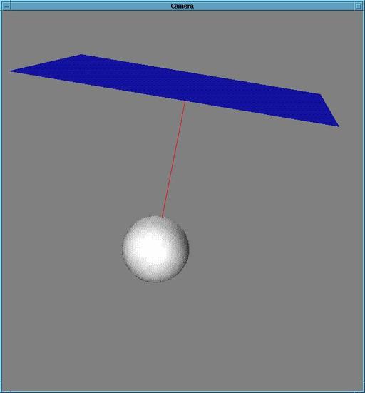
To see the results, compile the program with gcc pendulum.c. Next, start Geomview from this same directory and access the inspect menu and select commands. The command widget will pop up and you need to type (emodule-define pend a.out) to instruct Geomview to load the executable a.out as an external module named pend. If everything is working right, the module pend should appear in the external modules list and can be activated by clicking on the word pend. The pendulum and ceiling will appear in the camera widget and the pendulum will swing back and forth. You will have to use Geomview’s tools to rotate the scene to the view shown in Figure 3.

The loading of the OOGL object files and animation of the above example is accomplished in just a few lines of C code and a total of 4 GCL commands. The first two GCL commands describe some characteristics of the “World” (g0) object which, in turn, are adopted by all objects that are loaded following these commands. By default, when an object is loaded into Geomview, the coordinates of the object are normalized so that the object fits within a unit sphere centered on the origin. The (normalization g0 none) command turns this option off. The second command tells Geomview not to draw black bounding boxes around each object that it loads. The third command, (load filename), tells Geomview to load the OOGL object file filename.

Most of the work is actually done by the fourth and final GCL command. transform tells Geomview to rotate the object pendulum.list by 0.017 radians (about 1 degree) around the x axis and 0 radians about the y and z axes. The other two arguments to transform, g0 and focus, specify that rotations are with respect to the center of the World object (g0) and are to be applied in the frame of reference of the camera. There are many other GCL commands described in the manual that can be used to animate and manipulate OOGL objects.

Although the examples illustrated here have been rather simple, it should be apparent that Geomview is a package with numerous applications. Geomview, in combination with powerful graphical user interface development tools, such as Tcl and Wish, can be used to create interactive 3-D applications in relatively short amounts of time. This is quite a powerful package that should not be ignored by anyone developing applications involving 3-D images or anyone needing an easy-to-use viewer to better visualize objects, whether he is viewing complex mathematical output from Mathematica or simple geometric relationships between lines and planes.

You can find Geomview in several locations, including Sunsite. However, the home of Geomview is the anonymous ftp site ftp.geom.umn.edu. The Linux port can be found at pub/software/geomview/geomview-linux.tar.gz (3.1 MB). Source code, geomview-src.tar.gz, is available in the same directory.

If you have Netscape or Mosaic, I strongly recommend that you visit Geomview’s World Wide Web site, which is located at www.geom.umn.edu/software/download/geomview.html. At this site you will find not only executable code, but also an on-line tutorial for OOGL file formats, an FAQ, and introductions to other software. (While you are there, be sure to check out their Interactive Web Applications at www.geom.umn.edu/apps/.)

After Geomview is unpacked, it will occupy approximately 8.3 MB on your disk, including about 1 MB of documentation and 2.2 MB of examples. Unzipping and untarring will result in a new directory called Geomview. Change to this directory, read the README, and type install. The install script will ask you questions about where you want to install the executable, the manual pages, etc. At the end of the script, it will ask if you mind that the install script mails a registration to the Geometry Center. If you do not mind and have a mail facility set up on your machine, install will register you and place you on a very quiet mailing list (So far I have received only the registration confirmation).