 Linux, Linux OS, Free Linux Operating System, Linux India Linux, Linux OS,Free Linux Operating System,Linux India supports Linux users in India, Free Software on Linux OS, Linux India helps to growth Linux OS in India
All that is real is reasonable, and all that is reasonable is real. —G.W.F. Hegel, 1770-1831
Scientists and engineers were among the first to notice what a powerful combination the Linux kernel and the GNU tools are. Thus, it is no surprise that it was the sober scientists who started replacing expensive supercomputers with inexpensive networks of GNU/Linux systems. In spite of the strong position of GNU/Linux in all areas of scientific computing, there are still some aspects of the Linux kernel which have been neglected by engineers. One of them is the sound card interface.
In the early days of Linux, sound cards were notoriously unreliable in their ability to process data and continuous signals. They were supposed to handle sounds in games, and nothing more; few people tried to record data with them. Today, modern sound cards allow for simultaneous measurement of signals and control of processes in real time, and good sound cards can compete with expensive data acquisition cards which cost more than the surrounding PC. This article demonstrates how to abuse a sound card for measurements in the field.
With appropriate software, an ordinary PC can do much more than just record data in the field and analyse it off-line in the office. Due to the extreme computing power of modern CPUs, it is possible to analyse data while recording it in real time. On-line analysis allows for interactive exploration of the environment in the field, just like oscilloscopes of earlier days, but with an added dimension.
Sound Installation
Installing a sound card has always been a tricky task, whether you used MS-DOS, Windows or Linux. In the age of the PCI bus and Plug & Play (PnP), things have become much simpler, except for the many owners of legacy ISA bus cards with or without PnP.
The first place to go for help should always be the book that comes with your Linux distribution. They are usually very instructive, and should be taken seriously and not ignored. If you still encounter problems, have a look at the HOWTOs mentioned below. Different users have different needs; therefore, we have at least three different sources for sound drivers, each one addressing a different group of users.
- The commercial OSS (Open Sound System) has a very simple and secure installation procedure. Separate versions for SMP kernels and PCI cards are available. If you are not interested in buzzwords like PCI, ISA or PnP, and do not bother to pay for support, buy this one and you are done.
- OSS/free comes as part of the regular kernel. Alan Cox keeps an eye on it and has integrated many drivers for ISA cards, and also a few PCI cards. These drivers should also work with SMP. Kernel 2.4 will probably allow for sound production without a sound card; only a digital USB speaker will be needed.
- The Advanced Linux Sound Architecture (ALSA) project provides a free (but compatible) alternative to the different flavours of OSS. It supports some ISA and a few PCI cards. ALSA drivers have a clean, modular design for multiple sound cards and SMP, but they are still in the experimental stage. Do not try to install them unless you know how to compile and install a kernel and modular drivers.
For industrial applications, it is important that the sound drivers support SMP (symmetrical multiprocessing). SMP allows Linux to schedule processes in machines with two or more CPUs on their main board. Most of the drivers already support SMP. The most recent versions of OSS and ALSA also support multiple sound cards in one PC. The ALSA project has received some funding from SuSE, and their drivers will be integrated into the regular kernel. This will not happen before version 2.5 (experimental) of the kernel.
Fortunately, the Linux community has produced some very helpful documents (see Resources). Read them; you will benefit, and each one deserves to be read. There are also many applications (mixers, recorders, players, converters, synthesizers) available for free (see Resources).
First, you will need to install the sound card and its drivers in your Linux system. As usual, the book that comes with your Linux distribution should help a lot, and HOWTOs on the Internet provide the necessary instructions (see sidebar “Sound Installation”). When your sound card and its drivers are installed, you should do some testing with it. Make a recording while adjusting the mixer gain, and play the recording back through your loudspeaker. The mixer is an important feature of your sound card, because it allows you to adjust the sensitivity of the A/D converter to the level of the signal to be recorded. This is even more important when recording with a resolution of 8 bits. Keep in mind that we are looking for fast and robust measures of qualitative effects, rather than precise quantitative measurements.
Phase Space
In mathematics, the art of questioning often is more important than the art of solving a problem. —Georg Cantor, 1845-1918
Measuring a series of values in the field makes sense only if something actually happens, i.e., if there is some change to be seen. In a pendulum that has come to rest, there is not much to be measured. To start some action, we need a force; for example, someone giving the pendulum a push. After that, there are two independent forces that keep the pendulum swinging: inertia keeps it moving, while gravity pulls it down.
Only if two such forces act on the same body (thereby acting on each other in an opposing way) can cyclic motion occur. When the pendulum is at its largest displacement from its initial (at rest) position, it is at rest again for a short moment (velocity = 0 in Figure 3). All the energy from the initial push happens to be conserved in potential energy.
During each cycle, all the potential energy is first transformed completely into kinetic energy (at the bottom of the pendulum’s arc) and then back again into potential energy. Instead of graphing each of the two independent variables (displacement and velocity) over time, it is sometimes advantageous to graph them against each other, thereby eliminating the time axis (Figure 1) and revealing the cyclic nature of the process. This is derivative phase space.
What is phase space good for? If you know the values of both variables (displacement and velocity) at any time, you can make a pretty good guess about future values simply by following the closed curve in Figure 1. In case of noisy measurements (as in Figure 2), take the average motion.
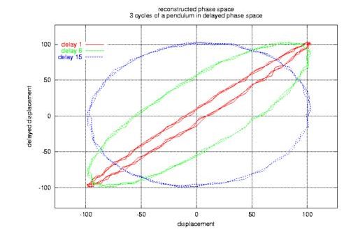
Most of the time, we can measure only one of the variables (displacement), losing the other one. Hence, we need to somehow reconstruct the lost variable (velocity) from the measured one. This can be done by graphing the measured variable against a delayed copy of itself, i.e., the displacement at time t on one axis and displacement at time t-tau on the other axis. This works surprisingly well if the delay is chosen properly, as in Figure 5.
If your GNU/Linux system does not already have some audio applications installed, see Resources for a collection of addresses on the Internet. There, you will find applications like smix, a mixer with a well-designed user interface. It can handle multiple sound cards, and has the features needed for serious work:
- interactive graphical user interface
- command-line interface
- configuration file settings
It makes no difference to your sound card whether the recorded signal comes from an acoustic microphone or an industrial sensor. Signals of any origin are always stored as sequences of values, measured at fixed time intervals (i.e., equidistant in time). Acoustic signals on a CD, for example, are sampled 44,100 times per second, resulting in one (stereo) value every 1/44100 = 22.7 microseconds.
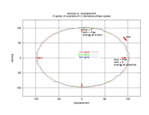
Figure 1. Phase Space Portrait of a Pendulum
While musicians may be interested in filtering these signals digitally (thereby distorting them), we are more interested in finding and analysing properties of the measured, undistorted signal. We are striving to find the rules of change governing the sampled series of values. The major tool in Nonlinear Signal Processing for finding the laws of motion is delay coordinate embedding, which creates a so-called phase space portrait from a single time series (Figures 1 and 2). If you are not interested in technical details, you may envisage it as a tool which turns a sequence of sampled numbers into a spatial curve, with each direction in space representing one independent variable. If you are interested in technical details, you will find them in the Phase Space sidebar. In any case, you should look at the list of FAQs of the newsgroup sci.nonlinear (see Resources). These explain the basic concepts and some misconceptions, and provide sources for further reading.
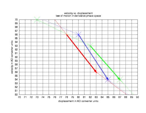
Figure 2. Progress of the Pendulum in Phase Space
Before delving into multi-dimensional space, let us look at an example. Plug a microphone into your sound card’s jack, whistle into the microphone and use any of the many freely available sound editors (see Resources) to record the whistling. The resulting recording will look very much like the sine wave in Figure 3. It is not surprising that your recorded wave form looks similar to the wave form of the pendulum in Figure 3. The vibrating substances (gas or solid) may be different, but the laws of motion are very similar; thus, the same wave form.
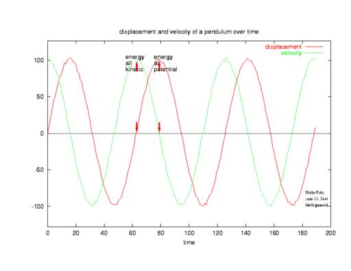
Figure 3. Wave Form of Pendulum
You can download some software from the FTP server of Linux Journal, which records your whistling and does the phase-space analysis for you (see Resources). Instead of displaying the wave form, the software just extracts important measures of the signal which help you refine your measurements (Figure 4). Remember, it is not my objective to show you how to present stunning, glossy pictures; rather, it is to demonstrate what a valuable tool your Linux machine is when analysing real-world signals in the field.
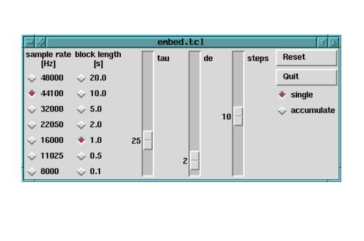
Figure 4. Finding a Good Embedding by Adjusting Independent Parameters
Start the software by typing
wish -f embed.tcl | dmm
A window will pop up that looks like Figure 4. In this window, you can control the way the software measures the whistling sound from your microphone. You can change the sample rate (click on 44,100Hz) from left to right, the length of the analysed blocks (click on 1 second) and the parameters tau and de, which are needed for reconstruction of the phase space portrait from just one measured signal. This is comparable to the displacement of Figure 1; we have no velocity measurement here.
Embedding
Those who have knowledge, don’t predict. Those who predict, don’t have knowledge. —Lao Tzu, 6th-century B.C. Chinese poet
The pendulum we are looking at in Figure 1 obviously has a phase-space portrait (a circle) that fits nicely onto a two-dimensional plane. The reconstructed phase portrait in Figure 5 is also a round curve without intersections. No doubt this is a valid and useful reconstruction. But what if the system in the field has more than two variables, and perhaps their interdependence is not so smooth? While our pendulum simply goes around and around in phase space, there may be other mechanisms with three independent variables, needing three dimensions in their original phase space. Even worse, their portrait may look more like a roller coaster than a flat circle. During the 1980s, scientists worked on this more general problem and found methods and justifications to deal with the situation:
- Can delayed phase space reconstruct the original phase space in all cases? Yes, but only if some inevitable requirements are met. There must be significant interaction among variables, otherwise the influence of a (weak) variable may get lost. Furthermore, a weak interaction may get lost in the presence of environmental noise.
- How many dimensions must the reconstructed phase space have? Choosing too low a dimension for delayed phase space can lead to “flattened” curves with intersections. Fortunately, topologists proved a theorem giving an upper bound: if the mechanism has n independent variables, a delayed phase space with 2n+1 variables can always avoid intersections. In most cases, fewer are necessary. This is called the embedding dimension de (always an integer).
- What are good values for tau and de, yielding a good reconstruction? There is no general way of telling in advance which values to use. However, many algorithms have been developed to judge the quality of given parameters tau and de. A popular one is the False Nearest Neighbours algorithm. It looks at a given delayed-phase portrait, and remembers which points are neighbours. If these points are no longer close to each other after increasing de, then the current de looks insufficient.
One of the most common mistakes among practitioners of the 1980s was using a fixed tau without thinking about it. If the quality of your data is questionable (because of a bad reconstruction or noise of any origin), it makes no sense to chase for signs of chaos.
Each time we analyse an unknown signal, we have to start with some educated guessing of the two parameters:
- tau is the temporal distance, or delay, between spatial coordinates
- de is the number of dimensions of the reconstructed phase space
These parameters are of crucial importance for a good unfolding of the portrait of the signal in reconstructed phase space (see the sidebar Embedding). In Figure 5, you can see how the choice of tau influences the portrait. Values which are too small cannot unfold the portrait; values which are too large are not shown, but often lead to meaningless (noisy, uncorrelated) portraits. The software supports you in finding good values for tau and de. After years of intense research, scientists still rely on some heuristics for choosing suitable values for these parameters.
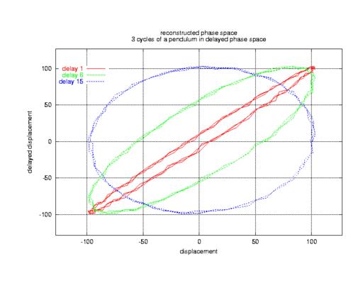
Figure 5. Differences in Unfolding, Depending on Parameter
In the particular case of your whistling, the values in Figure 4 should result in a good unfolding of the portrait. Do not worry about the text lines which fill your terminal window. They are needed for checking the quality of the unfolding. Restart the software by typing
wish -f embed.tcl | dmm | wish -f out.tcl
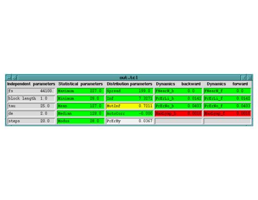
Figure 6. Parameters of a Sine Wave
and the text lines will be converted into the more readable form of Figure 6. In the additional window popping up now, you will see several columns. On the left (in grey), the independent parameters of the first window are repeated. The second column from the left tells you if the loudness of the measured signal is well-adjusted to the sensitivity of your sound card’s input. The general rule is, as long as there are red lines in the second column, you have to adjust sensitivity (with a separate mixer software) or loudness. Now, turning to the third column, we see more-advanced parameters:
- Spread is the difference between the largest and the smallest value, measured in AD converter units. Small values indicate insufficient strength of the signal.
- Inf is the average information content of one sample, measured in bits. A constant baseline signal yields 0 bits (minimum) and random noise has 8 bits (the maximum with 8-bit samples).
- MutInf is the average mutual information of one sample and the delayed one. Thus, it tells you how similar the signals of both axes in Figure 5 are. A value of 1 means they are perfectly coupled (in the sense of probabilistic dependency), 0 means completely independent.
- AutoCorr (autocorrelation) is another measure of similarity. Since the late 1980s, there has been a (questionable) rule of thumb saying that a value near 0 indicates a good unfolding of the reconstructed portrait. The maximum is 1.
- PrErHy measures predictability and therefore determinism of the signal. The underlying algorithm of prediction is the conventional linear predictive filter as used in many adaptive filtering applications like modems. The minimum 0 indicates perfect (linear) predictability, while the maximum 1 indicates complete unpredictability by means of linear filtering.
Determinism, Prediction and Filtering
Prediction is very difficult, especially of the future. —Niels Bohr, 1885-1962
How do we know whether our recorded signal is a deterministic signal or just noise? In the case of our recorded sine wave, the orderly behaviour is obvious from the graph over time (Figure 3). In the general case, it is easier to discover determinism in phase space (Figure 1). Look at a specific point in phase space, for example in Figure 2. Determinism means if the swinging system ever returns to the vicinity of this point, we can tell the next step in advance. Given the same circumstances again, the pendulum is determined to advance in the same way. A nondeterministic system may hop around like mad.
This understanding of deterministic behaviour rests on some assumptions:
- Precise measurement: but, our measurements are always noisy. Taking the average of the three motions in Figure 2 will improve the quality of prediction significantly.
- Adequate phase space: if the next step of the system depends on an additional variable (like total energy), the direction of progress might not be uniquely determined. This corresponds to a curve which could not be unfolded due to an insufficient reconstruction of phase space.
- Locality: this simple scheme works only if our measurement uses a fine resolution in time and space. Small steps in time and space tend to be locally bounded, allowing for easier detection of deterministic behaviour.
Prediction is always error-prone, and it makes sense to calculate the extent of failure. A comparison of deviation to the signal’s range is appropriate. Averaging all the local prediction errors produces a robust quantity for the estimation of the quality called determinism.
Building upon this reasoning, there is a wide range of applications. Adaptive linear predictive filtering is a very important paradigm in contemporary digital signal processing. Noise removal, speech and image compression and feature extraction are examples. Nonlinear generalizations of these applications are now feasible.
Again, the rule is, as long as there are red lines in the third column, phase space is not reconstructed properly. Now, turning to the last two columns, you will notice they look identical. Indeed, they are. The difference is this: when evaluating the parameters of the fourth column, the software uses a reversed time axis. When reversing time, i.e., exchanging past and future, prediction turns into postdiction and vice versa. Reversing the time axis is a simple and effective way of checking the validity of parameters which are especially susceptible to measurement errors. In general, if reversal of time changes a parameter, it is not trustworthy, which bring us to the next parameter:
- If FNearN (percentage of false nearest neighbours) is reliable, the lines will turn green and be the same in both columns (near 0). Otherwise, it will turn red and indicate that the neighbourship relation of points in phase space is not preserved when changing the parameter de, indicating an insufficient embedding.
- PrErLi is the result of re-calculating parameter PrErHy over the whole data block. They should always be roughly the same. If not, there must be a reason for it, and things get interesting.
- PrErN measures the predictability with a nonlinear prediction algorithm. Signals originating from a linear system are usually predicted more precisely by PrErLi while signals from nonlinear sources are often predicted better by nonlinear prediction.
- MaxLyap measures separation (progressing over time) of points nearby in phase space. By definition, values larger than 0 indicate chaos.
When measuring signals from nonlinear systems, PrErLi often turns red (indicating insufficient linear predictability) while PrErN stays green (indicating sufficient nonlinear predictability). In case of a truly chaotic signal, MaxLyap will turn green (valid) and have opposite signs on the right-most columns. This indicates nearby points are separating over time when time is going forward, and they are approaching each other at the same rate when moving backward in time.
Phase Space
In mathematics, the art of questioning often is more important than the art of solving a problem. —Georg Cantor, 1845-1918
Measuring a series of values in the field makes sense only if something actually happens, i.e., if there is some change to be seen. In a pendulum that has come to rest, there is not much to be measured. To start some action, we need a force; for example, someone giving the pendulum a push. After that, there are two independent forces that keep the pendulum swinging: inertia keeps it moving, while gravity pulls it down.
Only if two such forces act on the same body (thereby acting on each other in an opposing way) can cyclic motion occur. When the pendulum is at its largest displacement from its initial (at rest) position, it is at rest again for a short moment (velocity = 0 in Figure 3). All the energy from the initial push happens to be conserved in potential energy.
During each cycle, all the potential energy is first transformed completely into kinetic energy (at the bottom of the pendulum’s arc) and then back again into potential energy. Instead of graphing each of the two independent variables (displacement and velocity) over time, it is sometimes advantageous to graph them against each other, thereby eliminating the time axis (Figure 1) and revealing the cyclic nature of the process. This is derivative phase space.
What is phase space good for? If you know the values of both variables (displacement and velocity) at any time, you can make a pretty good guess about future values simply by following the closed curve in Figure 1. In case of noisy measurements (as in Figure 2), take the average motion.
Most of the time, we can measure only one of the variables (displacement), losing the other one. Hence, we need to somehow reconstruct the lost variable (velocity) from the measured one. This can be done by graphing the measured variable against a delayed copy of itself, i.e., the displacement at time t on one axis and displacement at time t-tau on the other axis. This works surprisingly well if the delay is chosen properly, as in Figure 5.
For the moment, the number of parameters and values may be overwhelming. If you start by playing with the software and actually analysing some signals in the field, you will soon become acquainted with the parameters in their colours and columns. The first time, you should look only at the two left-most columns in Figure 6. All parameters there have intuitive meanings, and you will soon be able to foretell how they change when applied to a different signal, a clipped signal or an oversampled signal. Here are some typical situations and how to recognize them:
- Sine wave: just as in Figure 6, de (embedding dimension) should be 2 or 3. Mean (i.e., average) and Median (i.e., “middlest”) are the same. Modus is jumping back and forth between Maximum and Minimum. If the Spread reaches its maximum (256), Inf gets near 8 (bits).
- Zero baseline (short-circuit or switched off) can be recognized by looking at column 2. All values are identical. In column 3, Spread and Inf are almost 0.
- Switching on a microphone, there is a short and sharp impulse resulting in a sudden change of Spread; few others change.
- Sawtooth (Figure 7) looks much like the sine, except for Modus, which jumps wildly. MutInf is at its maximum, linear prediction works only with higher-order filters, while nonlinear prediction works better with low embedding dimensions.
- Noise comes in many different flavours, all of them having low values of AutoCorr and most with a low MutInf.
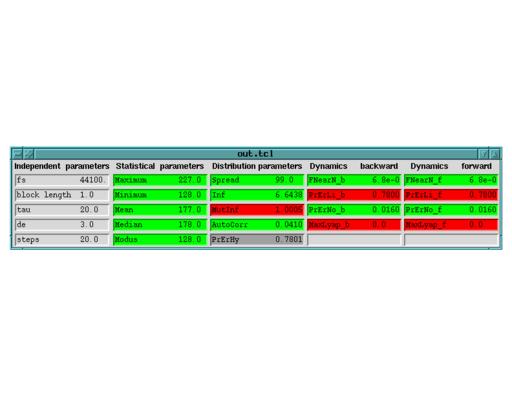
Figure 7. Parameters of a Sawtooth Signal
Why not calculate some kind of fractal dimension of a signal? By definition, calculation of dimensions must look at the values over a wide range of scales. With 8 bits of resolution, this is impossible or questionable. But even if we had some fractal dimension value, it would not be as useful as the largest Lyapunov exponent. Furthermore, are all these measurements any good? Yes, there are some areas of application:
- System Identification: in some applications, the focus of attention is more on the quality of the signal (stochastic or deterministic, linear or nonlinear, chaotic or not).
- Prediction: today, linear prediction is one of the most important algorithms for digital signal processors (DSPs) in telecommunication, be it mobile telephony, modems or noise canceling. If there are systems with nonlinear behaviour involved, nonlinear prediction can be advantageous (see sidebar “Determinism, Prediction & Filtering”).
- Control: if you know the structure of your system’s phase space well enough, you can try to control the system like this:
- Identify periodic orbits in phase space.
- Look for an orbit which meets the given requirements (goes through a certain point, or has minimum energy or cost).
- Modify a suitable parameter or a variable just slightly to stabilize the desired periodic orbit.
- When Ott, Grebogi & Yorke first published successful application of this method (called the OGY method) in 1990, they even managed to control a system in the presence of chaos.
Projects
The 1980s were the decade which drew the attention of scientists to nonlinear and chaotic phenomena. Scientists had to lay the groundwork by integrating geometric and topological concepts (phase space, embedding, Lyapunov exponents, dimensions). The 1990s were the decade of refinement and application. From an engineer’s point of view, there are at least three outstanding books worth mentioning which summarize the state of the art. Each book is supplemented by software for -line analysis, implementing the ideas presented in the respective books.
- Abarbanel was among the first to speak of a new applied discipline (Nonlinear Signal Processing) and outline it. You can find his book at http://www.zweb.com/apnonlin/. The software is called cspX TOOLS FOR DYNAMICS. It is commercial software and can be found at http://www.zweb.com/apnonlin/csp.html.
- Kantz & Schreiber name the discipline and their book Nonlinear Time Series Analysis. Their software is called TISEAN. It is free and can be found at http://www.mpipks-dresden.mpg.de/~tisean/. TISEAN 2.0 is also available for the MS Win32 platforms, because they compiled it with the Cygwin Toolset, the free UNIX emulation layer on top of Win32.
- Nusse & Yorke distribute their software (called Dynamics2) with their book (called Dynamics 2nd Ed.). It is a hands-on approach to learning the concepts and computing relevant quantities: http://keck2.umd.edu/dynamics/general_info/smalldyn_download.html.
In the list of FAQs of sci.nonlinear, you will find even more books, links and software (see Resources).
In the late 1990s, several people analysed the time series of the financial markets in order to find signs of nonlinearity or chaos (for example, Blake LeBaron in Weigend & Gershenfeld’s book, page 457). Some hoped to be able to predict time series of stock values in this way. Kantz & Schreiber took the idea one step further, and contemplated the application of the OGY method to control the stock market. But in a footnote on page 223 of their book, they admit, “We are not aware of any attempts to control the stock market as yet, though.” When I looked at the chart of Red Hat stock in late 1999, I wondered whether someone had finally managed to apply the OGY method to the time series of the Red Hat share price.